A Robotics Ecosystem made for Python.
A Pythonic, open-source, and modern Robotics suite.
import spatialmath as sm
sm.SE3.Rx(1.0)

    1         0         0         0
    0         0.5403   -0.8415    0
    0         0.8415    0.5403    0
    0         0         0         1
import roboticstoolbox as rtb
rtb.models.Panda()
ERobot: panda (by Franka Emika), 7 joints (RRRRRRR), 1 gripper, geometry, collision
┌─────┬──────────────┬───────┬─────────────┬────────────────────────────────────────────────┐
│link │ link │ joint │ parent │ ETS: parent to link │
├─────┼──────────────┼───────┼─────────────┼────────────────────────────────────────────────┤
│ 0 │ panda_link0 │ │ BASE │ │
│ 1 │ panda_link1 │ 0 │ panda_link0 │ SE3(0, 0, 0.333) ⊕ Rz(q0) │
│ 2 │ panda_link2 │ 1 │ panda_link1 │ SE3(-90°, -0°, 0°) ⊕ Rz(q1) │
│ 3 │ panda_link3 │ 2 │ panda_link2 │ SE3(0, -0.316, 0; 90°, -0°, 0°) ⊕ Rz(q2) │
│ 4 │ panda_link4 │ 3 │ panda_link3 │ SE3(0.0825, 0, 0; 90°, -0°, 0°) ⊕ Rz(q3) │
│ 5 │ panda_link5 │ 4 │ panda_link4 │ SE3(-0.0825, 0.384, 0; -90°, -0°, 0°) ⊕ Rz(q4) │
│ 6 │ panda_link6 │ 5 │ panda_link5 │ SE3(90°, -0°, 0°) ⊕ Rz(q5) │
│ 7 │ panda_link7 │ 6 │ panda_link6 │ SE3(0.088, 0, 0; 90°, -0°, 0°) ⊕ Rz(q6) │
│ 8 │ @panda_link8 │ │ panda_link7 │ SE3(0, 0, 0.107) │
└─────┴──────────────┴───────┴─────────────┴────────────────────────────────────────────────┘
┌─────┬─────┬────────┬─────┬───────┬─────┬───────┬──────┐
│name │ q0 │ q1 │ q2 │ q3 │ q4 │ q5 │ q6 │
├─────┼─────┼────────┼─────┼───────┼─────┼───────┼──────┤
│ qr │ 0° │ -17.2° │ 0° │ -126° │ 0° │ 115° │ 45° │
│ qz │ 0° │ 0° │ 0° │ 0° │ 0° │ 0° │ 0° │
└─────┴─────┴────────┴─────┴───────┴─────┴───────┴──────┘
from swift import Swift
import roboticstoolbox as rtb
env = Swift()
env.launch()
panda = rtb.models.Panda()
env.add(panda)
from machinevisiontoolbox import Image
mona = Image.Read("monalisa.png")
Image.Hstack([mona, mona.smooth(sigma=5)]).disp()Comprehensive
The Python Robotics Ecosystem encompasses tools in manipulation, mobile robots, robotic vision, spatial mathemtics, simulation, and more.
Fast
We use C extensions in key places to enable lightning fast execution. Get forward kinematicsin less than 1µs and inverse kinematics in less than 20µs.
Pythonic
We follow the conventions and style set out by the Python community to produce software which is clear, consice, and easy to use.
Visualisations
We provide powerful visualisation tools to view the results of your algorithms through our simulator Swift and matplotlib.
The Robotics Toolbox for Python.
The Robotics Toolbox provides the robot-specific functionality and contributes tools for representing the kinematics and dynamics of manipulators, robot models, mobile robots, path planning algorithms, kinodynamic planning, localisation, map building and simultaneous localisation and mapping.
# Import the robotics toolbox
import roboticstoolbox as rtb

# Make a Panda robot
panda = rtb.models.Panda()

# Make a set of joint coordinates q
# (7 joint angles)
q = [0 , -0.3, 0, -2.2, 0, 2, 0.78]

# Compute the forward kinematics at q
fk = panda.fkine(q)

# Compute the (base frame) Jacobian at q
J = panda.jacob0(q)

# Print the results
print(f"The forward kienmatics is:\n {fk}")
print(f"\nThe Jacobian is:\n {J}")
The forward kinamtics at q is:
0.995 0 0.09983 0.484
0 -1 0 0
0.09983 0 -0.995 0.4126
0 0 0 1
The Jacobian at q is:
[[ 6.46597923e-17 7.96297755e-02 4.35044282e-17 2.46636972e-01
1.37144864e-17 2.00563536e-01 0.00000000e+00]
[ 4.84046815e-01 2.96393192e-17 4.85959793e-01 1.88781536e-17
1.54695257e-01 -1.20466388e-18 0.00000000e+00]
[ 1.23259516e-32 -4.84046815e-01 1.20663347e-17 4.98615940e-01
-1.41699602e-17 1.08565317e-01 0.00000000e+00]
[ 0.00000000e+00 -3.08148791e-33 -2.95520207e-01 -3.61907875e-17
9.46300088e-01 -3.61907875e-17 9.98334166e-02]
[ 2.46519033e-32 1.00000000e+00 2.73485128e-18 -1.00000000e+00
-1.13507164e-16 -1.00000000e+00 -1.20329446e-16]
[ 1.00000000e+00 6.12323400e-17 9.55336489e-01 5.57626374e-17
-3.23289567e-01 5.57626374e-17 -9.95004165e-01]]The Swift simulator and visualiser.
Swift is a robot simulator controlled by Python but displayed in a web browser using several web technologies, including React, Next.js, and Three.js. The entire simulator can be downloaded and installed from Python package managers PyPI or Conda-forge with no external downloads or installs.
# Import swift
from swift import Swift

# Import the robotics toolbox
import roboticstoolbox as rtb

# Make a Panda robot
panda = rtb.models.Panda()

# Set the joint angles of the robot
panda.q = [0 , -0.3, 0, -2.2, 0, 2, 0.78]

# Make and launch a Swift environment
env = Swift()
env.launch()

# Add the robot to the environment
env.add(panda)The Spatial Maths toolbox.
Spatial Maths provides the ability to describe objects' position, orientation or pose in 2D or 3D spaces -- this capability underpins all of robotics. This package supports the Special Euclidean groups, Special Orthogonal groups, quaternions, twists, and various mathematical operations and conversions between them.
# Import spatialmath
import spatialmath as sm

# Construct an SE(3) (a homogeneous transformation matrix) from a
# rotation about the z-axis
T1 = sm.SE3.Rz(1.0)
print(f"T1:\n{T1}")

# Convert Euler angles to an SE(3)
T2 = sm.SE3.Eul(0.1, 0.2, 0.3)
T2.printline()

# Construct an SE(3) from an x, y, z translation
T3 = sm.SE3.Trans(1.0, 2.0, 3.0)
T3.printline()

# Find the 3D transfromation from T1 to the inverse of T2 to T3
result = T1 * T2.inv() * T3
print(f"Result:\n{result}")

# Extract the rotation from the result to RPY
print(f"result RPY:\n{result.R}")T1:
0.5403 -0.8415 0 0
0.8415 0.5403 0 0
0 0 1 0
0 0 0 1
t = 0, 0, 0; rpy/zyx = 3.43°, 10.9°, 23.2°
t = 1, 2, 3; rpy/zyx = 0°, 0°, 0°
result:
0.8102 -0.5662 -0.152 -0.778
0.5519 0.8241 -0.128 1.816
0.1977 0.01983 0.9801 3.178
0 0 0 1
result RPY:
[ 0.02023447, -0.1989874 , 0.59798006]
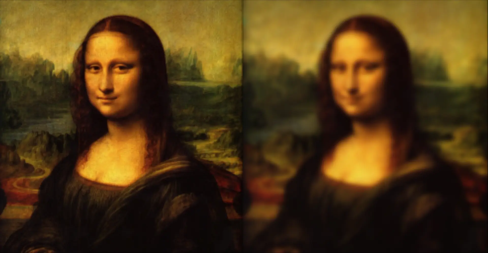
The Machine Vision toolbox.
The Machine Vision Toolbox provides many functions for robotic vision -- crucial for achieving robotics in the real-world. The included methods support monadic, dyadic, filtering, edge detection, mathematical morphology and feature extraction. A collection of camera projection classes for central (normal perspective), fisheye, catadioptric and spherical cameras. And some advanced algorithms in around multiview geometry, camera calibration, stereo vision, bundle adjustment, and bag of words.
# Import Image from the machine vision toolbox
from machinevisiontoolbox import Image
## Reading and displaying an Image
# Read an image from a file
mona = Image.Read("monalisa.png")
# Display the original and smoothed images side by side
Image.Hstack([mona, mona.smooth(sigma=5)]).disp()
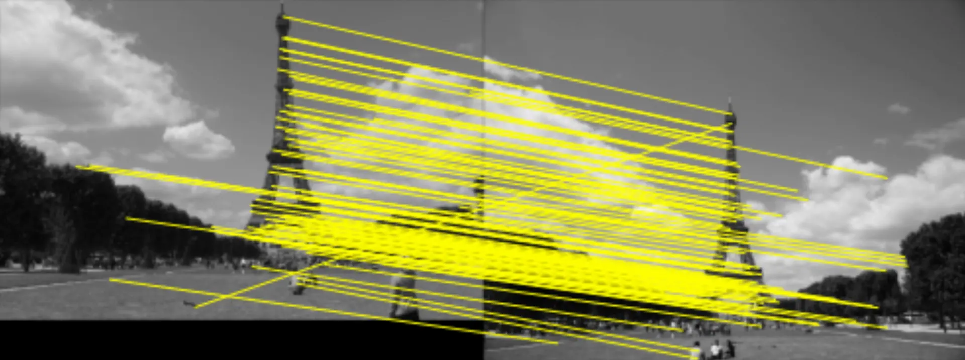
## SURF features
# Load two images and compute a set of SURF features for each
view1 = Image.Read("eiffel-1.png", mono=True)
view2 = Image.Read("eiffel-2.png", mono=True)
sf1 = view1.SIFT()
sf2 = view2.SIFT()
# Match features between images based purely on the similarity
matches = sf1.match(sf2)
# display the correspondences
matches.subset(100).plot("w")
Supported by Utility packages.
The Python Robotics ecosystem has strong foundations through our utility packages: Spatial Geometry, ANSItable and PGraph. Spatial Goemetry provides functionality for representing 3D geometry, pose graphs and collsion checking. We're big fans of console tools not GUIs but that doesn't mean we have do without graphics. The toolboxes use unicode characters and ANSItable helps create and display tables of data in a variety of formats. PGraph provides a class for creating, manipulating, and displaying of directed and non-directed graphs which are used for everthing from path planning to bundle adjustment.
import spatialgeometry as sg

# Make a cuboid and a sphere and check if they collide
cuboid = sg.Cuboid([1.0, 1.0, 1.0])
sphere = sg.Sphere(1.0)
print(cuboid.iscollided(sphere))
Trueimport ansitable
# Make and print a table
table = ANSITable(
"col1",
"column 2 long header",
"column 3",
border="thin")
table.row("medium long", 2.2, 3)
table.row("much longer than the other", 5.5, 6)
table.row("short", 8.8, 9)
table.print()
┌───────────────────────────┬──────────────────────┬──────────┐
│                      col1 │ column 2 long header │ column 3 │
├───────────────────────────┼──────────────────────┼──────────┤
│               medium long │                  2.2 │        3 │
│much longer than the other │                  5.5 │        6 │
│                     short │                  8.8 │        9 │
└───────────────────────────┴──────────────────────┴──────────┘
import pgraph as pg

## Make an undirected graph
# Make a new vertex class
class Foo(pg.UVertex):
    # foo stuff goes here
    pass

f1 = Foo()
f2 = Foo()

# Make the graph
g = pg.UGraph()
g.add_vertex(f1)
g.add_vertex(f2)

# Make and check the connections
f1.connect(f2, cost=3)
for f in f1.neighbours():
    print(f"connected to {f}")
connected to [#1]Perfectly Interoperable.
Each of our packages have been designed to work in perfect harmony with each other. This allows for a seamless integration of all of our packages into your project.
# Import packages
import roboticstoolbox as rtb
import spatialgeometry as sg
import spatialmath as sm

# Make a Panda robot
panda = rtb.models.Panda()

# Set a goal pose for the panda using Spatial Maths
Tep = sm.SE3.Trans(0.6, -0.3, 0.1) * \
    sm.SE3.OA([0, 1, 0], [0, 0, -1])

# Make a goal axes using Spatial Geometry and set to
# the goal pose
goal_ax = sg.Axes(0.1, pose=Tep)

# Use inverse kinematics to find the joint angles
# which achieve the goal
sol = panda.ikine_LM(Tep)

# Plot the robot at the solution in Swift
env = panda.plot(sol.q)

# Add our goal axes to the environment
env.add(goal_ax)
Community
See the code and get involved
By Jesse Haviland and Peter Corke
© Copyright 2022